
Processing Pipeline
Table of Contents
- Introduction
- Filter Layer
- Vector Field Computation
- Analysis Layer
- Debugging and Profiling (Server Application)
- Performance and Stability
Introduction
The extraction of user interactions takes place mainly in the filtering and analysis layer; accordingly, the processing of sensor data is divided into two pipeline sections of the same name. The starting point is the point cloud calculated from the sensor data, which contains the actual depth points in a two-dimensional array. In addition to the world coordinates (X, Y, Z), these also contain two flags each, which determine whether the points are valid and whether they have been modified by a filter. The indices of the array correspond to the rows and columns of the sensor image.
Filter Layer
Some filters use an incremental filtering method: instead of being replaced by a default value, values affected by the filtering are reset to the measured value from the previous measurement. In the case of static effects, this is equivalent to resetting to a default value, as the point cloud is initialised with default values. In the case of temporary disturbances, this prevents additional disturbances from being introduced. The filtering process consists of a sequence of different transformation steps applied to the point cloud to clean and smooth the sensor values. Specifically, the following filters are applied:
- Truncation of the value range (LimitiationFilter): In the basic implementation, the point cloud is truncated at the edges based on minimum and maximum values for the row and column indices. The aim is to remove areas outside the elastic surface, in the event that the sensor’s detection range extends beyond it. In the case of the Microsoft Azure Kinect sensor, an additional challenge was that the camera image does not capture a rectangular area but rather an octagonal shape. Consequently, the filter was extended to include a masking function. The indices of the masked areas are filtered out of the point cloud. Values that fall outside the valid range when the filter is applied are marked as invalid.
- Handling missing data (ValueFilter): This incremental filter detects missing values and resets them to the previous measured value.
- Handling outliers (ThresholdFilter): This incremental filter checks whether the distance to the previous position exceeds a predefined threshold and resets the value accordingly.
- Smoothing (BoxFilter): The simplest implementation of smoothing uses a box filter, which filters out high-frequency components by calculating a moving average. Thanks to the simple calculation and the ability to separate the filter axes, the box filter offers a good compromise between speed and quality. Approximating a Gaussian filter by applying it in several passes yields better results with only a slight increase in computational effort. This version of the filter can be further accelerated by distributing the work across different threads.
The final step in the pipeline involves updating the depth values in the stored point cloud and, based on this, calculating the vector field.
Vector Field Computation
The use of the detected surface deformation in the form of a vector field requires the depth values to be transformed into direction vectors. As the point cloud is available as an elevation map with a regular grid, this is achieved by simply calculating the gradient for each point. This is done by calculating the differences between neighbouring Z-values in the x and y directions. The difference is normalised based on the horizontal and vertical distances, respectively, between the neighbouring points.
An offset can be applied to reduce the resolution of the vector field, thereby minimising the number of calculation steps. The vectors at the edge of the point cloud, for which no neighbouring points exist in a given direction, are set to zero vectors.
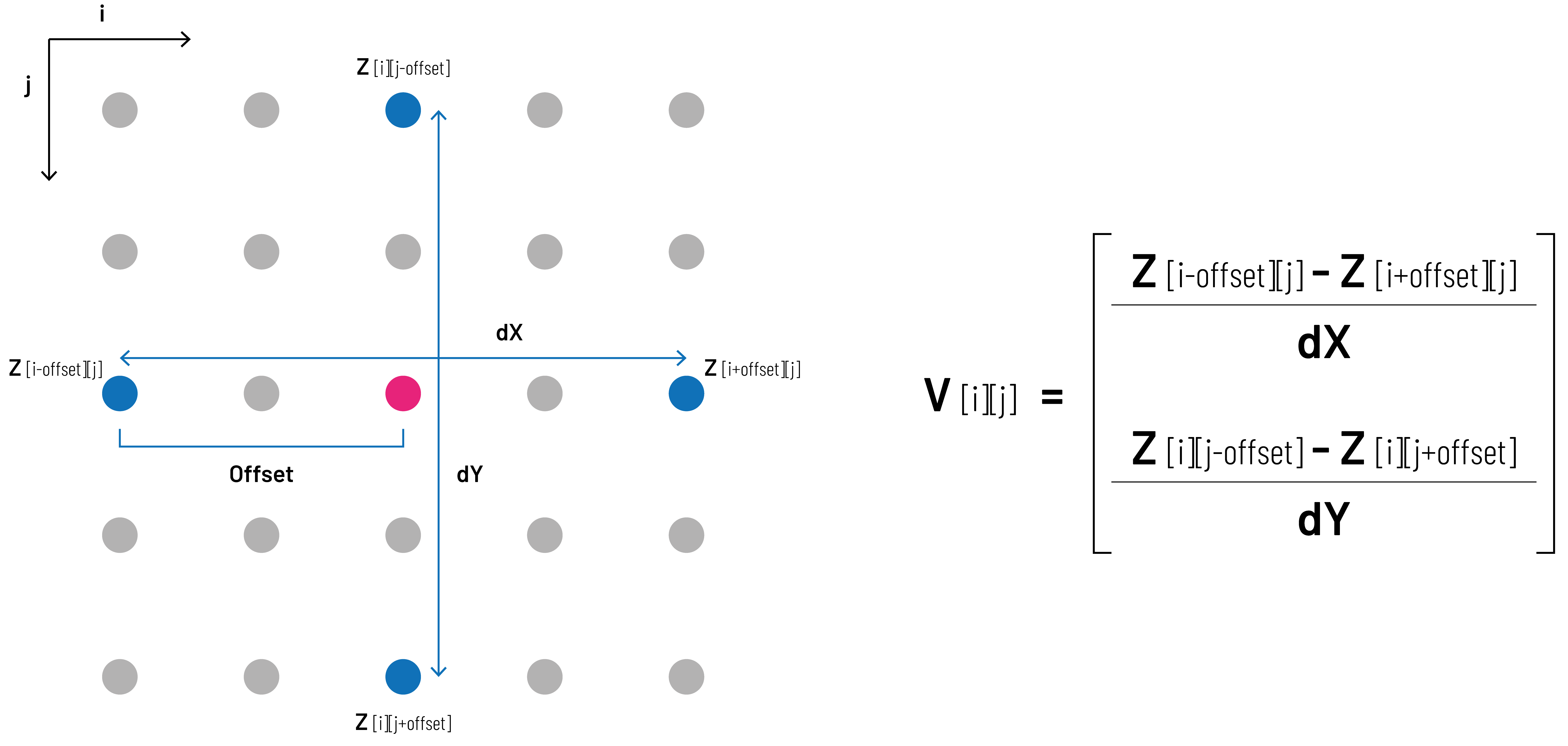
A common computational approach involves including the differences to more distant points in the calculation, weighted according to a Gaussian distribution; this would correspond to filtering the vector field with a Gaussian filter. However, from the perspective of the total number of computational steps, this is problematic and, due to the upstream filtering of the point cloud, redundant. Filtering the point cloud also has the advantage that smoothing can be carried out more efficiently using an algorithm with a separable kernel (such as a Box filter or a Gaussian filter) than if this were integrated into the calculation of the vector field.
The stability of the vector field is improved by means of temporal smoothing, whereby the calculated values are temporarily stored and then combined with the newly determined values in the subsequent frame using a weighting factor. By default, a fixed factor of 0.7 is used for the current value, whilst the most recently stored value is factored in with a weighting of 0.3. With this method, the influence of values from further back is also retained, albeit with a decreasing weight.
Analysis Layer
The analysis phase basically extracts the touch interactions based on the vector field and comprises up to five steps:
- Pre-processing (Preparation): In this optional step, the point cloud is converted into a usable format or its resolution is reduced to speed up the calculation. In the current implementation, this step is only relevant when using an external service as part of the analysis.
- Extraction of extreme values (Analyse): Depending on the selected modality, this step involves calculating either the global extreme value (single-touch) in the point cloud or the local extrema based on the vector field, and assigning confidence values to them (multi-touch, see Section 7.2.3). The iteration of the vector field is optimised through parallelised processing. Additionally, the resolution of the vector field can be reduced by skipping values in order to improve performance. This reduction in resolution affects the accuracy of the user interaction’s position. The risk of outliers being filtered out by this approach is low, as only high-frequency outliers based on signal noise are removed. However, as these have already been largely eliminated by previous filtering, this effect is negligible.
- Normalisation of the depth value (ConvertDepth): The extracted extreme values contain the world coordinates in the sensor’s coordinate system. In the first step, the depth values are mapped to the configured interaction area. Here, the value 0 corresponds to the normal plane, the value -1 corresponds to the maximum depth when pressing into the surface, and +1 to the maximum deflection when pulling away. The lateral positions remain in the world coordinate system for the time being.
- Classification and validation of extreme values (ExtremumType): In this step, the type of extreme value is first determined. When using multi-touch detection, this is followed by a classification to determine whether the event is a user interaction or an implicit extremum. Implicit extrema are then removed.
- Smoothing and Touch-ID Assignment (Smoothing*): Finally, the depth values are (optionally) smoothed and the corresponding Touch-ID is reconstructed.
Before the interaction points are finally transmitted, the lateral coordinates are converted from the sensor coordinate system to the projection coordinate system on the basis of the available calibration data. These are then converted into normalised coordinates. The transmitted 3D points are normalised to the range [0, 1] for the X and Y components and [-1, 1] for the Z component.
Debugging and Profiling (Server Application)
The server application includes a 3D view of the filtered point cloud that can be rotated and zoomed. Among other things, the points invalidated by filtering are visible and are displayed in red. In addition, the normal plane and the maximum deflection of the surface are displayed as planes. Furthermore, a bounding box for all elements of the point cloud (including filtered ones) can be displayed to assess whether the sensor is detecting elements outside the table or wall that could be potential sources of error. The detected interaction points are visualised to enable an assessment of the accuracy of the detection. For sensor alignment, the position of the point cloud in relation to the room axes is also relevant; this can be determined from the 3D view.
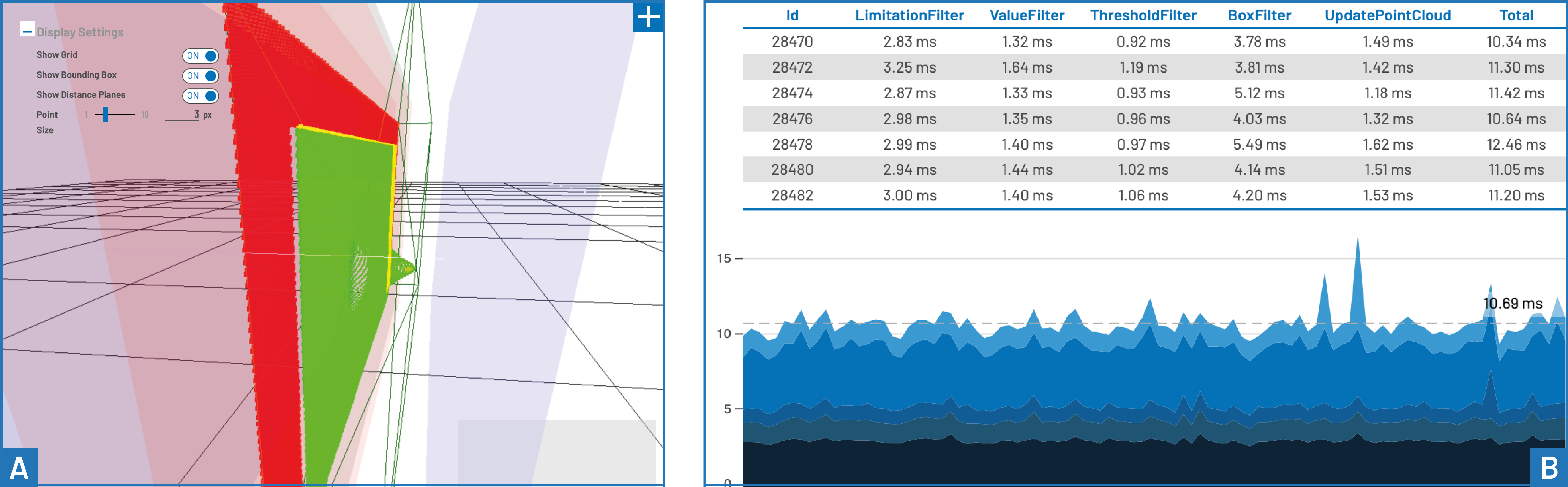
Furthermore, a visualisation of performance data is provided to give an impression of the stability of the processing. This is based on standard profiling tools used in modern 3D engines.
Performance and Stability
Perfomance and stability of the processing pipeline have beeen validated in real-world use of the framework. During a public demonstration in June 2025, measurements of the duration of the individual processing steps were carried out continuously throughout the entire duration of over 6 hours.
Version 0.9.9 of the framework was used. The following hardware components were utilised:
| CPU | AMD Ryzen 7 5800X |
| RAM | 32 GB |
| GPU | nVidia GeForce RTX 4070 |
| HDD | 1 TB SSD |
| OS | Microsoft Windows 11 |
| Sensor | Microsoft Azure Kinect DK (SDK-Version: 1.4.2) |
After cleaning the data sets, 425,974 recorded frames remained for the recording period. Without examining the results in detail, these data indicate an average frame rate of 19.44 frames per second and an average latency of 51.44 ms between individual frames (Duration: 06:05:12 = 21,912 s, 425,974 frames / 21,912 s = 19.440 frames/s). The descriptive statistics below provide an overview of the key metrics (All numbers represent miliseconds).
| Metric | Median | Mean | SD | min | max |
|---|---|---|---|---|---|
| Frame duration (Client) | 47.47 | 51.44 | 16.669 | 4.70 | 1200.06 |
| Pipeline complete | 18.95 | 24.32 | 16.854 | 3.38 | 1462.01 |
| Filter complete | 14.19 | 17.29 | 11.020 | 0.00 | 1166.91 |
| LimitationFilter | 5.80 | 6.66 | 4.050 | 0.00 | 502.99 |
| ValueFilter | 1.44 | 1.74 | 2.154 | 0.00 | 565.59 |
| ThresholdFilter | 1.10 | 1.38 | 2.030 | 0.00 | 357.70 |
| BoxFilter | 3.65 | 4.63 | 5.607 | 0.00 | 1155.71 |
| Update | 1.88 | 2.88 | 6.626 | 0.00 | 1127.46 |
| Analysis complete | 4.47 | 7.03 | 11.464 | 2.44 | 1098.52 |
| Analysis | 4.18 | 6.74 | 11.422 | 0.00 | 1098.23 |
| ConvertDepth | 0.11 | 0.13 | 0.720 | 0.00 | 429.91 |
| ExtremumType | 0.01 | 0.01 | 0.042 | 0.00 | 20.00 |
| Smoothing | 0.11 | 0.16 | 0.576 | 0.01 | 157.19 |
Frame duration measures the total time that elapses on the client side between two frames, and thus includes sensor latency and the processing time of the pipeline. Over the entire runtime, this averages 51.44 ms (SD = 16.669 ms, median = 47.47 ms, 95% CI = [51.399 ms, 51.499 ms]). Apart from a few significant outliers, the processing consistently delivers good frame times. In total, 6,346 frames had a duration of more than 100 ms for this metric, which corresponds to 1.490 per cent of the recorded data.
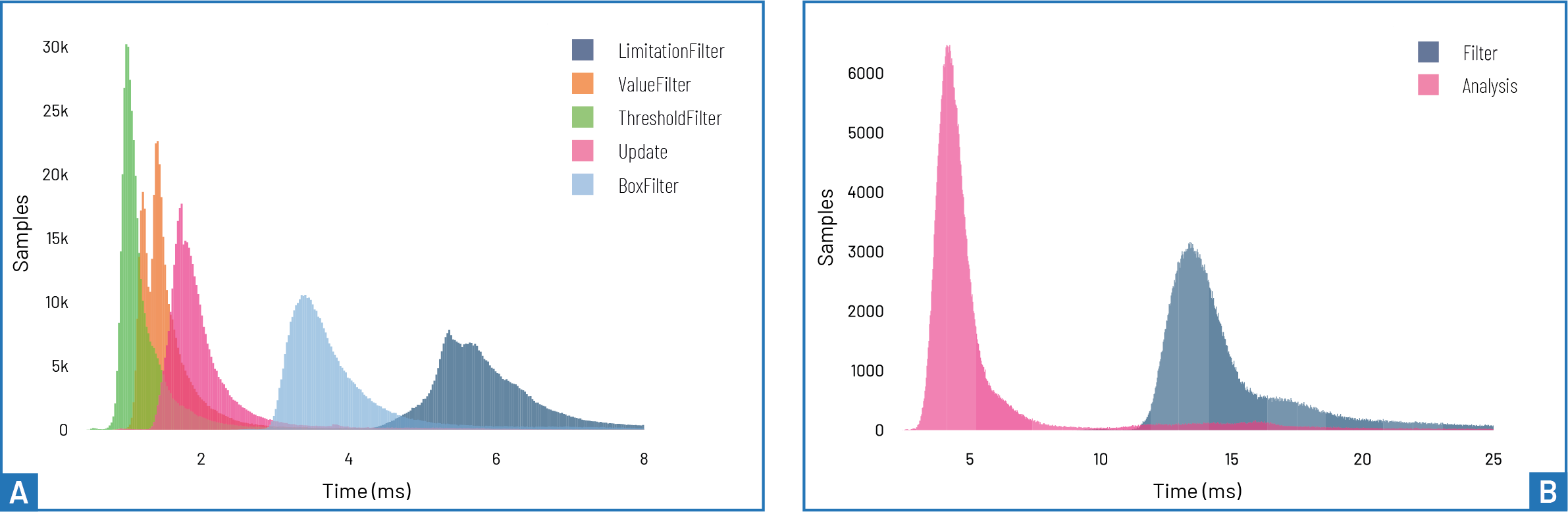
The average processing time of the pipeline was 24.32 ms (SD = 16.854 ms, median = 18.95 ms, 95% CI = [24.269 ms, 24.370 ms]). Here, too, the times are stable. However, alongside a comparatively small number of outliers, a larger number of times in the mid-range were observed. Specifically, this means that the number of frames in which the pipeline execution took more than 100 ms was very low, at 3,533 frames (= 0.829 per cent of the total data series). When considering the target of 50 ms, however, a significantly larger number of data points are affected (18,571 frames, 4.360 per cent of the data).